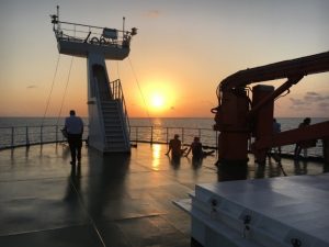
 The weather remains good, the sea is calm and we are about to cross the equator for the third time. We are steaming westward away from Africa and have some long transits between stations. Time to enjoy the sunsets and sunrises. But, this has also given us some time to start acquiring magnetic data.
Electromagnetic induction is behind many geophysical methods. Movement of a magnet can induce an electric current, and vice versa – this is the basis of the magnetotelluric method … but more on this later. The rapid movement of liquid iron in the outer core – by rapid, I mean as fast as a snail moves – gives rise to the Earth’s magnetic field. This field shields us from harmful stellar winds, but also provides us with a means of navigation, as the needle on a compass points towards the North Magnetic Pole.
Ships have played an important role in our study of the Earth’s magnetic field. Historical records of declination (the angle between geographical north and magnetic north) and inclination (the angle between horizontal and the dip of a compass needle) of the magnetic field have allowed geomagnetists to model how the field has varied in time, which in turn tells us something about dynamic mechanisms of the Earth’s outer core that lead to a magnetic field. The position of the magnetic pole is constantly changing and there is a westward drift of anomalies at the equator. As a historical note, the first maps of magnetic declination were produced in 1702 by Edmond Halley, based on extensive measurements by ships in the Atlantic.
One of the crucial bits of evidence that lent support to the idea of plate tectonics involved evidence of geomagnetic pole reversals in the geologic record. These reversals occur at irregular intervals roughly every few 100’s thousands to millions of years, but happen very rapidly (over 1000s of years). The rocks of the sea floor are strongly magnetic and their remnant magnetism after formation acts like a time stamp on the new crust produced at an oceanic spreading centre (in our case, the Mid-Atlantic Ridge). Magnetic surveys as early as the 1950s showed clear linear patterns in magnetic anomalies on the sea floor, but it was not until the 1960s that these observations were tied to the idea of new plates being formed at mid-ocean ridges, which are more correctly termed oceanic spreading centres.
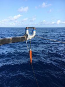
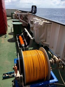
Even though this is now a very routine measurement at sea, for me, it is exciting given the historical context of the technique. So, I was up at 3am to help Martin, the research technician from the National Oceanography Centre, deploy the instrument with Johnny Mac, the scientific Bosun.
 We are using a type of proton precession magnetometer, which is towed over 300m behind the ship. As a rule of thumb, magnetometers are towed 3 ship lengths behind the winch to get away from the magnetic signal of the metal in the ship. A current is passed through a coil that is wrapped around a proton-rich canister of fluid (e.g. water or kerosene). The hydrogen protons align with the field induced by the coil. The current is then turned off and the protons precess back to the direction of the Earth’s magnetic field. The frequency of precession is proportional to the strength of the magnetic field. Our magnetometer uses something known as the ‘Overhauser effect’, which I think removes the need for orienting the sensors – but as we have virtually no access to the internet, I cannot check.
Our magnetometer is towed off the port-side of the ship and flies at a depth of roughly 6m when we are doing 10 knots. The manufacturer describes the instrument rather flowerly as a ‘surveyor’s best friend’, with ‘unfailing data, durable hardware, and an easy-going disposition’. I must admit it is easy to use and the data look reasonable. Looking a bit like a fish, sea-borne magnetometers often return with shark’s teeth in them.